It could be said that if you go to the grocery store and buy some Captain Crunch (once my favorite cereal) you would also be more likely to buy milk. Association Rules are if/then statements that help uncover relationships between seemingly unrelated data in a relational database or other information repository. They find all sets of items (itemsets) that have support greater than the minimum support and then use the large itemsets to generate the desired rules that have confidence greater than the minimum confidence. The lift of a rule is the ratio of the observed support to that expected if X and Y were independent.  A typical and widely used example of association rules application is market basket analysis. For example, if a customer buys a pair of running shoes, she is 75% more likely to also purchase running socks.

The symbol “” means implies, so the rule above is “if X the likely Y”. So, in our example, the rule would be “Buys Running Shoes Buys Running Socks”. So, an association rule has two parts, an antecedent (if) and a consequent (then). An antecedent is an item found in the data. A consequent is an item that is found in combination with the antecedent.

Association rules are created by analyzing data for frequent if/then patterns and using the criteria support and confidence to identify the most important relationships. Support is an indication of how frequently the items appear in the database. Confidence indicates the number of times the if/then statements have been found to be true.

In data analytics, association rules are useful for analyzing and predicting customer behavior. They play an important part in shopping basket data analysis, product clustering, catalog design and store layout.

Example:

AIS Algorithm

The AIS algorithm [1] was the first algorithm proposed by Agrawal, Imielinski, and Swami for mining association rule. It focuses on improving the quality of databases together with necessary functionality to process decision support queries. In this algorithm only one item consequent association rules are generated, which means that the consequent of those rules only contain one item, for example, rules like X ∩ Y ⇒ Z can be generated but not the rules like X ⇒ Y ∩ Z (“∩” is set notation for AND).

The databases were scanned many times to get the frequent item sets in AIS. To make this algorithm more efficient, an estimation method was introduced to prune those itemset candidates that have no hope to be large, consequently the unnecessary effort of counting those item sets can be avoided. Since all the candidate itemsets and frequent itemsets are assumed to be stored in the main memory, memory management is also proposed for AIS when memory is not enough.

In AIS algorithm, the frequent itemsets were generated by scanning the databases several times. The support count of each individual item was accumulated during the first pass over the database. Based on the minimal support count those items whose support count less than its minimum value gets eliminated from the list of item. Candidate 2-itemsets are generated by extending frequent 1-itemsets with other items in the transaction.

During the second pass over the database, the support count of those candidate 2-itemsets are accumulated and checked against the support threshold. Similarly those candidate (k + 1)-itemsets are generated by extending frequent k-itemsets with items in the same transaction. The candidate itemsets generation and frequent itemsets generation process iterate until any one of them becomes empty.

In summary:

1. Candidate itemsets are generated and counted on-the-fly as the database is scanned.
2. For each transaction, it is determined which of the large itemsets of the previous pass are contained in this transaction.
3. New candidate itemsets are generated by extending these large itemsets with other items in this transaction.

The disadvantage of the AIS algorithm is that it results in unnecessarily generating and counting too many candidate itemsets that turn out to be small.

SETM (Set Oriented Mining) Algorithm

The SETM algorithm was motivated by the desire to use SQL to compute large itemsets [2, 3]. C_k represents the set of candidate itemsets in which the Transaction Identity (TID) of the generating transactions has been associated with the itemsets. Each member of these sets is of the form < TID, itemset>. The TID uniquely identifies each transaction, much like a primary key in a database table. In SETM algorithm, candidate itemsets are generated on the fly as the database is scanned. After reading a transaction, it is determined which of the itemsets that were found to be frequent in the previous pass are contained in this transaction. New candidate itemsets are generated by extending these frequent itemsets with other items in the transaction. A frequent itemset L is extended with only those items that are frequent and occur later in the lexicographic ordering of items than any of the items in L.

The candidates generated from a transaction are added to the set of candidate itemsets maintained for the pass. In order to use the standard SQL join operation for candidate generation, SETM separates candidate generation from counting. It saves a copy of the candidate itemset together with the TID of the generating transaction in a sequential structure (such as a temporary table).

At the end of the pass, the support count of candidate itemsets is determined by sorting and aggregating this sequential structure.

SETM remembers the TIDs of the generating transactions with the candidate itemsets. To avoid the need of a subset operation, it uses this information to determine the frequent itemsets contained in the transaction read.

The final relation C_k is obtained by deleting those candidates that do not have minimum support. Assuming that the database is sorted in TID order, SETM can easily find the frequent itemsets contained in a transaction in the next pass by sorting the data by TID. In fact, it needs to visit every member of C_k only once in the TID order, and the candidate generation can be performed using the relational merge-join operation.

In summary:

1. Candidate itemsets are generated on-the-fly as the database is scanned, but counted at the end of the pass.
2. New candidate itemsets are generated the same way as in AIS algorithm, but the TID of the generating transaction is saved with the candidate itemset in a sequential structure.
3. At the end of the pass, the support count of candidate itemsets is determined by aggregating this sequential structure.

The SETM algorithm has the same disadvantage of the AIS algorithm. Another disadvantage is that for each candidate itemset, there are as many entries as its support value.

Apriori Algorithm

Apriori [4] is the best-known algorithm to mine association rules. It uses a breadth-first search strategy to count the support of itemsets and uses a candidate generation function which exploits the downward closure property of support. The Apriori algorithm makes multiple passes over the database. In the first pass individual item support is counted and the items that have support greater than or equal to minimum support are considered as large items. For each pass k after that, the large itemsets in the previous pass is grouped in sets of k items and these form candidate itemsets. The support for the different candidate itemsets is counted and if the support is found to be greater than minimum support then that itemset is considered to be large. This process continues until the large itemset in a particular pass comes out to be an empty set.

In summary:

1. Candidate itemsets are generated using only the large itemsets of the previous pass without considering the transactions in the database.
2. The large itemset of the previous pass is joined with itself to generate all itemsets whose size is higher by 1.
3. Each generated itemset that has a subset which is not large is deleted. The remaining itemsets are the candidate ones.

The Apriori algorithm takes advantage of the fact that any subset of a frequent itemset is also a frequent itemset. The algorithm can therefore, reduce the number of candidates being considered by only exploring the itemsets whose support count is greater than the minimum support count. All infrequent itemsets can be pruned if it has an infrequent subset.

AprioriTid Algorithm

Similar to the Apriori algorithm, the AprioriTid algorithm also uses the apriori-candidate generation function to determine the candidate itemsets but the difference is that the database is not used for counting support after the first pass [5]. Instead, sets of candidate itemsets are used for this purpose for k > 1. In case a transaction does not have any candidate k-itemset then the set of candidate itemsets would not have any entry for that transaction which will eventually decrease the number of transactions in the set containing the candidate itemsets as compared to the database. As value of k increases each entry will be smaller than the corresponding transactions because the number of candidates in the transactions will decrease. Apriori performs better than AprioriTid in the initial passes but in the later passes AprioriTid has better performance than Apriori. Due to this reason we can use another algorithm called Apriori Hybrid algorithm in which Apriori is used in the initial passes but we switch to AprioriTid in the later passes.

In summary:

1. The database is not used at all for counting the support of candidate itemsets after the first pass.
2. The candidate itemsets are generated the same way as in Apriori algorithm.
3. Another set C’ is generated of which each member has the TID of each transaction and the large itemsets present in this transaction. This set is used to count the support of each candidate itemset.

The advantage is that the number of entries in C’ may be smaller than the number of transactions in the database, especially in the later passes.

AprioriHybrid Algorithm

Apriori does better than AprioriTid in the earlier passes. However, AprioriTid does better than Apriori in the later passes. Hence, a hybrid algorithm can be designed that uses Apriori in the initial passes and switches to AprioriTid when it expects that the set C’ will fit in memory [5].

Association Rules using R

This example requires the “Visualizing Categorical Data” (vcd) package and the datasets “Arthritis” and “HairEyeColor”.

> require(vcd)
Loading required package: vcd
Loading required package: grid
> data("Arthritis")
> tab <- xtabs(~Improved + Treatment, data = Arthritis)
> summary(assocstats(tab))
 
Call: xtabs(formula = ~Improved + Treatment, data = Arthritis)
Number of cases in table: 84
Number of factors: 2
Test for independence of all factors:
Chisq = 13.055, df = 2, p-value = 0.001463
X^2 df P(> X^2)
Likelihood Ratio 13.530 2 0.0011536
Pearson         13.055 2 0.0014626
 
Phi-Coefficient   : 0.394
Contingency Coeff.: 0.367
Cramer's V        : 0.394
 

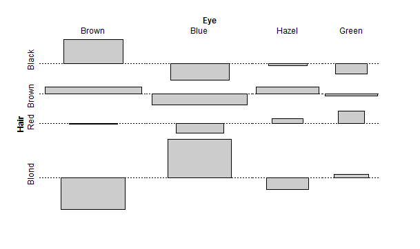
Next we compute a table margin. This is a contingency table in array form, computing the sum of table entries for a given index. Then we make a Cohen-Friendly association plot indicating deviations from independence of rows and columns in a 2-dimensional contingency table.  In the Cohen-Friendly association plot, each cell is represented by a rectangle that has (signed) height so that the area of the box is proportional to the difference in observed and expected frequencies. The rectangles in each row are positioned relative to a baseline indicating independence, when the Pearson’s Chi-square is zero. If the observed frequency of a cell is greater than the expected one, the box rises above the baseline and is shaded in the color specified by the first element of col, which defaults to black; otherwise, the box falls below the baseline and is shaded in the color specified by the second element of col, which defaults to red.

> ## Aggregate over sex:
> x <- margin.table(HairEyeColor, c(1, 2))
> x
Eye
Hair   Brown Blue Hazel Green
Black     68   20    15     5
Brown    119   84    54    29
Red       26   17    14    14
Blond      7   94    10    16

> assocplot(x, main = "Relation between hair and eye color")

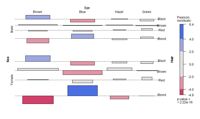
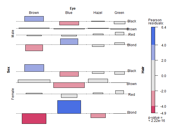
Next, we produce an association plot indicating deviations from a specified independence model in a possibly high-dimensional contingency table. assoc is a generic function and currently has a default method and a formula interface. Both are high-level interfaces to the strucplot function, and produce (extended) association plots. Most of the functionality is described there, such as specification of the independence model, labeling, legend, spacing, shading, and other graphical parameters.  In the association plot, each cell is represented by a rectangle that has (signed) height proportional to the observed counts and width proportional to the square root of the expected counts, so that the area of the box is proportional to the difference in observed and expected frequencies. The rectangles in each row are positioned relative to a baseline indicating independence (Pearson’s Chi-square = 0). If the observed frequency of a cell is greater than the expected one, the box rises above the baseline, and falls below otherwise.

> data("HairEyeColor")
> ## Aggregate over sex:
> (x <- margin.table(HairEyeColor, c(1, 2)))
                        Eye
Hair   Brown Blue Hazel Green
Black     68   20    15     5
Brown    119   84    54    29
Red       26   17    14    14
Blond      7   94    10    16
>
> ## Ordinary assocplot:
> assoc(x)
> ## and with residual-based shading (of independence)
> assoc(x, main = "Relation between hair and eye color", shade = TRUE)

Our previous analysis or Hair Color and Eye Color was aggregated over sex. We now examine Hair Color and Sex aggregated over Eye Color.

> ## Aggregate over Eye color:
> (x <- margin.table(HairEyeColor, c(1, 3)))
                  Sex
Hair   Male Female
Black    56     52
Brown   143    143
Red      34     37
Blond    46     81
> chisq.test(x)
 
Pearson's Chi-squared test
 
data: x
X-squared = 7.9942, df = 3, p-value = 0.04613
 
> assoc(x, main = "Relation between hair color and sex", shade = TRUE)
> # Visualize multi-way table
> assoc(aperm(HairEyeColor), expected = ~ (Hair + Eye) * Sex,
+       labeling_args = list(just_labels = c(Eye = "left"),
+                           offset_labels = c(right = -0.5),
+                           offset_varnames = c(right = 1.2),
+                           rot_labels = c(right = 0),
+                          tl_varnames = c(Eye = TRUE))
+ )

Finally, we aggregate data on applicants to graduate school at Berkeley for the six largest departments in 1973 classified by admission and sex. The association plot will show the admissions by sex for hair color and eye color, which I suppose should lead us to ask questions like, “Do women with blond hair and brown eyes incur a disadvantage for being admitted?” 

> assoc(aperm(UCBAdmissions), expected = ~ (Admit + Gender) * Dept, compress = FALSE,
+       labeling_args = list(abbreviate = c(Gender = TRUE), rot_labels = 0)
+ )
 
> ## UCB Admissions
> data("UCBAdmissions")
> ucb <- aperm(UCBAdmissions)
>
> ## association plot for conditional independence
> strucplot(ucb, expected = ~ Dept * (Admit + Gender),
+           core = struc_assoc(ylim = c(-4, 4)), labeling_args = list(abbreviate = c(Admit = 3)))

Works Cited

1. Qiankun Zhao, Sourav S. Bhowmick, Association Rule Mining: A Survey, Technical Report, CAIS, Nanyang Technological University, Singapore, 2003
2. R. Rantzau, “Algorithms and applications for universal quantification in relational databases”, Information Systems,Vol. 28(1-2), March 2003.
3. M. A. W. Houtsma, A.N. Swami, “Set-oriented mining for association rules in relational databases”, ICDE 95 Proc. of the 11th International Conference on Data Engineering, IEEE Computer Society, pp. 25-33, 1995.
4. Agrawal, Rakesh; and Srikant, Ramakrishnan; Fast algorithms for mining association rules in large databases, in Bocca, Jorge B.; Jarke, Matthias; and Zaniolo, Carlo; editors, Proceedings of the 20th International Conference on Very Large Data Bases (VLDB), Santiago, Chile, September 1994, pages 487-499
5. Manisha Girotra, Kanika Nagpal Saloni inocha Neha Sharma Comparative Survey on Association Rule Mining Algorithms, International Journal of Computer Applications (0975 – 8887) Volume 84 – No 10, December 2013
   

   ---

   Authored by:
   Jeffrey Strickland, Ph.D.

   Jeffrey Strickland, Ph.D., is the Author of Predictive Analytics Using R and a Senior Analytics Scientist with Clarity Solution Group. He has performed predictive modeling, simulation and analysis for the Department of Defense, NASA, the Missile Defense Agency, and the Financial and Insurance Industries for over 20 years. Jeff is a Certified Modeling and Simulation professional (CMSP) and an Associate Systems Engineering Professional (ASEP). He has published nearly 200 blogs on LinkedIn, is also a frequently invited guest speaker and the author of 20 books including:

   • Operations Research using Open-Source Tools
   • Discrete Event simulation using ExtendSim
   • Crime Analysis and Mapping
   • Missile Flight Simulation
   • Mathematical Modeling of Warfare and Combat Phenomenon
   • Predictive Modeling and Analytics
   • Using Math to Defeat the Enemy
   • Verification and Validation for Modeling and Simulation
   • Simulation Conceptual Modeling
   • System Engineering Process and Practices

   Connect with Jeffrey Strickland
   Contact Jeffrey Strickland