Since I have been teaching data analytics in India for the past month, I have been searching for an example of text analytics using R. Several months ago I saw a demonstration on creating word clouds. The R packages tm, koRpus, and RTestTools seemed like promising choices. But I could never get the packages with their dependencies installed in R. Meanwhile, I drove forward and eventually required ggmap for a home value problem, which would also not load. Consequently, I updated my version of R and R Studio and applied the latest patch. After that, tm and wordcloud2 installed without difficulty. Yet, I could not find the example I witnessed months before. So, here is my version of using tm to create word clouds.

The Packages

The R packages required to perform the following tasks include tm, wordcloud2, yaml, ggplot2, and their dependencies. In R studio, you merely need to use the Tool | Install Packages… menu to perform this feat. Alternatively, you can use the R function install.packages(“package name”) at the R prompt. Once installed, we read them into R with using the function, library(package-name).

library(wordcloud2)
library(yaml)
library(NLP)
library(tm)
library(SnowballC)
library(ggplot2)

File Setup

On a PC, we save the folder to your C: drive and use the following code chunk (I am not certain how this is accomplished for the Mac OS):

cname <- file.path("C:/Users/Strickland/Documents/VIT University", "texts")
cname
dir(cname)
docs <- Corpus(DirSource(cname))
summary(docs)
inspect(docs)

Text Preparation

The following code removes all punctuation and special characters, respectively:

docs <- tm_map(docs, removePunctuation)
for(j in seq(docs))
{
docs[[j]] <- gsub("/", " ", docs[[j]])
docs[[j]] <- gsub("@", " ", docs[[j]])
docs[[j]] <- gsub("\\|", " ", docs[[j]])
}
inspect(docs[1])

Next, we remove numbers, “stopwords” (common words) that usually have no analytic value, and particular words, as well as converting the text to lowercase letters.

docs <- tm_map(docs, removeNumbers)
docs <- tm_map(docs, tolower)
docs <- tm_map(docs, removeWords, stopwords("english"))
docs <- tm_map(docs, removeWords, c("can", "should", "would", "figure", "using", "will", "use", "now", "see", "may", "given", "since", "want", "next", "like", "new", "one", "might", "without"))

We also want to combine words that should stay together:

for (j in seq(docs))
{
docs[[j]] <- gsub("data analytics", "data_analytics", docs[[j]])
docs[[j]] <- gsub("predictive models", "predictive_models", docs[[j]])
docs[[j]] <- gsub("predictive analytics", "predictive_analytics", docs[[j]])
docs[[j]] <- gsub("data science", "data_science", docs[[j]])
docs[[j]] <- gsub("operations research", "operations_research", docs[[j]])
docs[[j]] <- gsub("chi-square", "chi_square", docs[[j]])
}

Now, we remove common word endings (e.g., “ing”, “es”, “s”), and strip unnecessary whitespace from our documents:

docs <- tm_map(docs, stemDocument)
docs <- tm_map(docs, stripWhitespace)

The next commands tells R  to (1) treat our preprocessed documents as text documents, (2) create a document term matrix, and (3) create a transpose of the previously created matrix.

docs <- tm_map(docs, PlainTextDocument)
dtm <- DocumentTermMatrix(docs)
tdm <- TermDocumentMatrix(docs)

Word Frequency Analysis

The next code tells R organizes the terms by their frequency and print a matrix to be saved as a .csv file.

freq <- colSums(as.matrix(dtm))
length(freq)
ord <- order(freq)
m <- as.matrix(dtm)
dim(m)
write.csv(m, file="dtm.csv")

Next, we get ready to analyze the text for word frequencies. We start by removing sparse terms. This makes a matrix that is 10% empty space, maximum:

dtms <- removeSparseTerms(dtm, 0.1)
inspect(dtms)

Next, we check some of the frequency counts. There are a lot of terms, so for now, we just check out some of the most and least frequently occurring words, as well as check out the frequency of frequencies.

freq[head(ord)]
freq[tail(ord)]
head(table(freq), 50)
tail(table(freq), 50)
freq <- colSums(as.matrix(dtms))
freq <- sort(colSums(as.matrix(dtm)), decreasing=TRUE)
head(freq, 14)
findFreqTerms(dtm, lowfreq=150)

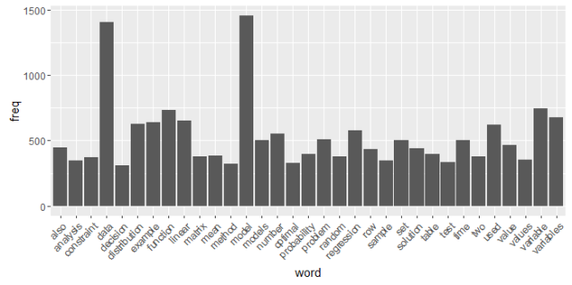
Frequency Plotting

Now we put the last created frequency into a data frame and use ggplot to render a histogram of word frequencies. We are looking for frequency counts of at least 300, but you can adjust the count to fit your needs:

wf <- data.frame(word=names(freq), freq=freq)
head(wf)
p <- ggplot(subset(wf, freq>300), aes(word, freq))
p <- p + geom_bar(stat="identity")
p <- p + theme(axis.text.x=element_text(angle=45, hjust=1))
p

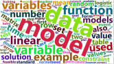
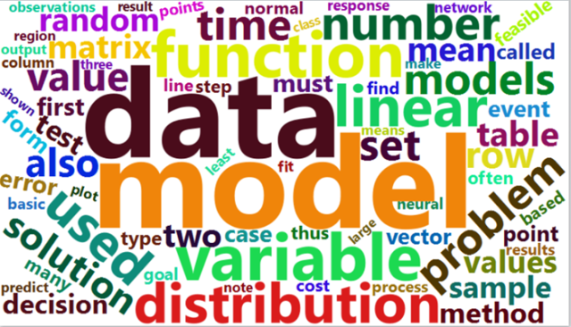
Finally, we create the Word Cloud:

wordcloud2(subset(wf, freq>50))

Other tasks, like correlations, can be easily performed with the tm package.

Jeffrey Strickland, Ph.D.

Jeffrey Strickland, Ph.D., is the Author of Predictive Analytics Using R and a Senior Analytics Scientist with Clarity Solution Group. He has performed predictive modeling, simulation and analysis for the Department of Defense, NASA, the Missile Defense Agency, and the Financial and Insurance Industries for over 20 years. Jeff is a Certified Modeling and Simulation professional (CMSP) and an Associate Systems Engineering Professional (ASEP). He has published nearly 200 blogs on LinkedIn, is also a frequently invited guest speaker and the author of 20 books including:

• Data Analytics using Open-Source Tools
• Operations Research using Open-Source Tools
• Discrete Event simulation using ExtendSim
• Crime Analysis and Mapping
• Missile Flight Simulation
• Mathematical Modeling of Warfare and Combat Phenomenon
• Predictive Modeling and Analytics
• Using Math to Defeat the Enemy
• Verification and Validation for Modeling and Simulation
• Simulation Conceptual Modeling
• System Engineering Process and Practices

Connect with Jeffrey Strickland
Contact Jeffrey Strickland